Google Sheets
Lesson 13: Creating Complex Formulas
Introduction
You may have experience working with formulas that contain only one operator, such as 7+9. More complex formulas can contain several mathematical operators, such as 5+2*8. When there's more than one operation in a formula, the order of operations tells Google Sheets which operation to calculate first. To write formulas that will give you the correct answer, you'll need to understand the order of operations.
Watch the video below to learn how to create complex formulas.
Order of operations
Google Sheets calculates formulas based on the following order of operations:
- Operations enclosed in parentheses
- Exponential calculations (3^2, for example)
- Multiplication and division, whichever comes first
- Addition and subtraction, whichever comes first
A mnemonic that can help you remember the order is Please Excuse My Dear Aunt Sally.
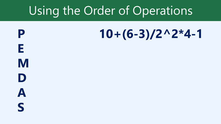
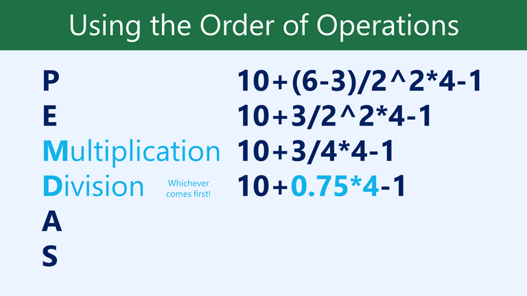
While this formula may look complicated, we can use the order of operations step by step to find the right answer.
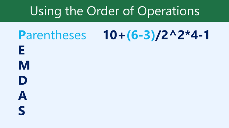
First, we'll start by calculating anything inside parentheses. In this case, there's only one thing we need to calculate: 6-3=3.

As you can see, the formula already looks simpler. Next, we'll look to see if there are any exponents. There is one: 2^2=4.
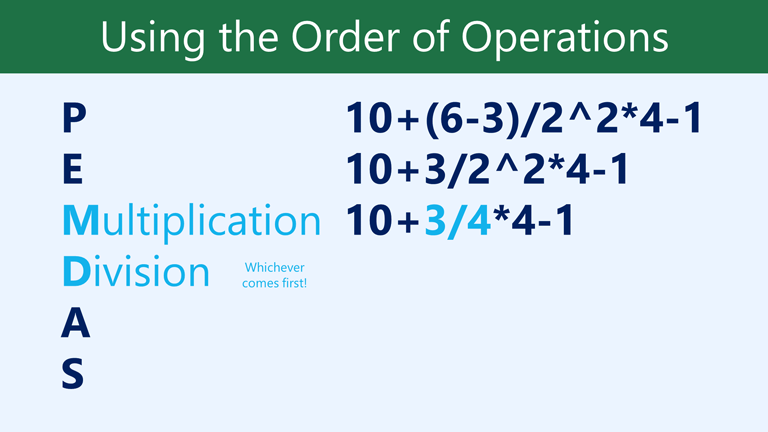
Next, we'll solve any multiplication and division, working from left to right. Because the division operation comes before the multiplication, it's calculated first: 3/4=0.75.
Now, we'll solve our remaining multiplication operation: 0.75*4=3.
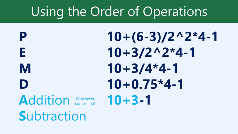
Next, we'll calculate any addition or subtraction, again working from left to right. Addition comes first: 10+3=13.
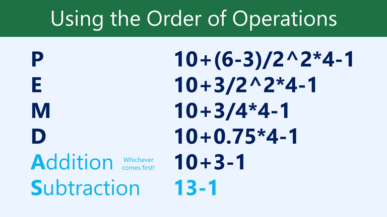
Finally, we have one remaining subtraction operation: 13-1=12.
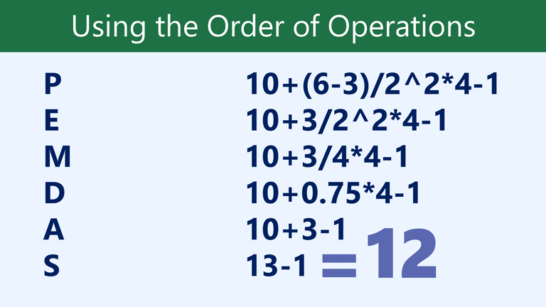
Now we have our answer: 12. And this is the exact same result you would get if you entered the formula into Excel.

Creating complex formulas
In the example below, we'll demonstrate how Google Sheets solves a complex formula using the order of operations. The complex formula in cell D6 calculates the sales tax by adding the prices together and multiplying by the 5.5% tax rate (which is written as 0.055).
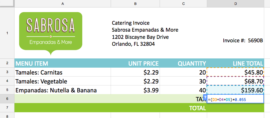
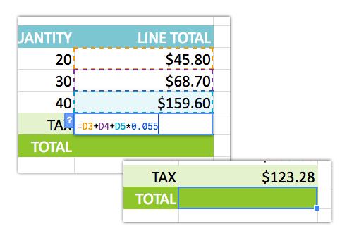
Google Sheets follows the order of operations and first adds the values inside the parentheses: (D3+D4+D5) = $274.10. Then it multiplies by the tax rate: $274.10*0.055. The result will show that the tax is $15.08.

It's especially important to follow the order of operations when creating a formula. Otherwise, Google Sheets won't calculate the results accurately. In our example, if the parentheses are not included, the multiplication is calculated first and the result is incorrect. Parentheses are often the best way to define which calculations will be performed first in Google Sheets.
To create a complex formula using the order of operations:
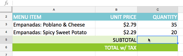
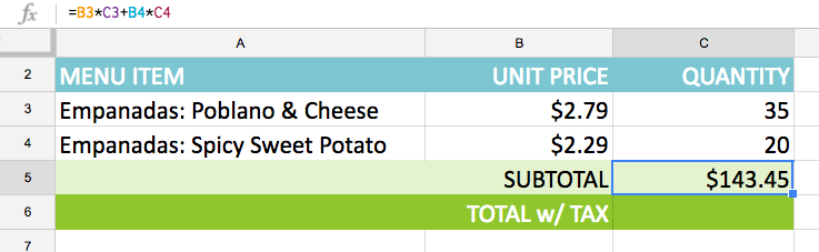
In the example below, we'll use cell references along with numerical values to create a complex formula that will calculate the subtotal for a catering invoice. The formula will calculate the cost of each menu item first, then add these values.
- Select the cell that will contain the formula. In our example, we'll select cell C5.
- Enter your formula. In our example, we'll type =B3*C3+B4*C4. This formula will follow the order of operations, first performing the multiplication: 2.79*35 = 97.65 and 2.29*20 = 45.80. It then will add these values to calculate the total: 97.65+45.80.
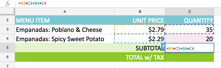
- Double-check your formula for accuracy, then press Enter on your keyboard. The formula will calculate and display the result. In our example, the result shows that the subtotal for the order is $143.45.
Google Sheets will not always tell you if your formula contains an error, so it's up to you to check all of your formulas. To learn how to do this, read our article on why you should Double-Check Your Formulas.
Challenge!
- Open our example file. Make sure you're signed in to Google, then click File > Make a copy.
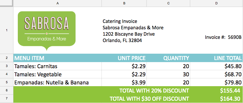
- Select the Challenge sheet. Let's say we want to compare two discounts. The first discount takes 20% off the total, and the second discount takes $30 off the total.
- In cell D6, create a formula that calculates the total using the 20% off discount.
Hint: Because we're taking 20% off, 80% of the total will remain. To calculate this, multiply 0.80 by the sum of the line totals. - In cell D7, create a formula that subtracts 30 from the total.
- When you're finished, your spreadsheet should look like this: